July 30, 2024

AI Meets Mechanobiology: Decoding the Mechanics of Living Systems
Shailaja Seetharaman, Eric and Wendy Schmidt AI in Science Postdoctoral Fellow
Mechanical forces are everywhere. From blood flow through arteries to pressure in the airways, and we are continuously sensing and responding to such varying stimuli. Whether it is a single cell sensing its local microenvironment or us as a whole reacting to external stimuli, forces orchestrate form and function. For example, shear stress in blood vessels is crucial for cardiovascular health, while in cancer, extracellular matrix stiffness affects tumor growth and metastasis. However, the mechanisms by which mechanical cues orchestrate tissue functions remain elusive. Introducing new approaches from artificial intelligence (AI) and machine learning (ML) with domain knowledge in biology, we can decode the mechanics of biological systems.

Figure 1. Endothelial tissue in response to changes in shear stress. Microscopy image of human aortic endothelial cells experiencing disturbed flow mimicking atherosclerosis in arteries. Cells are stained for actin (magenta), cell junctions/boundaries using VE-Cadherin (red), and a mechanosensitive protein called Four-and-a-half LIM domain protein 2 (FHL2; cyan).
Challenges in Biological Systems
When cells and tissues respond to forces, several events occur in parallel. Proteins move around within the cell, alter their interactions and signaling, resulting in drastic remodeling of subcellular structures like the nucleus and cytoskeleton. Some structures assemble and grow, while others disassemble. These molecular and subcellular events drive tissue-scale behaviors, leading to phenomena such as cell shape changes, cell adhesion and migration. Compared to physical systems where theoretical modeling has been very successful, engineering models for living systems are still a nascent stage.
Living systems are made up of thousands of different biological molecules that function with highly dynamic and non-linear interactions. Fundamentally, this means that our current modeling approaches and engineering disciplines that rely on studies of non-living systems will be inapplicable in biology. Furthermore, several AI “blackbox” models lack interpretability, and this is a critical problem, particularly when used to predict diseased states or patient health. Despite these challenges, AI holds immense potential in decoding vast biological data. AI algorithms can analyze large genomics/proteomics datasets and microscopy images to identify patterns and correlations, helping us develop targeted therapies to enhance precision medicine.
Harnessing AI in Cardiovascular Research
Understanding how force sensing and adaptation occurs in cardiovascular systems is an extremely important step towards identifying and designing targeted therapies for heart diseases. Inspired by the successes of AI in protein structure and interactions, drug design and digital pathology, researchers are exploring the potential of AI in mechanobiology. For example, machine learning models can detect subtle changes in signals that could indicate heart failure or atrial fibrillation.
As a Schmidt AI in Science Postdoctoral Fellow, I’ve been interested in exploiting AI/ML approaches in addressing one of the open problems in the field of vascular mechanobiology, namely, how blood flow variations in diseases like atherosclerosis impact tissue phenotypes and functions. Specifically, we are predicting how cardiac endothelial cells respond to laminar blood flow in healthy arteries or turbulent flow seen in diseases like atherosclerosis. Using machine learning tools and high-throughput methods to model how proteins, subcellular structures, and tissues behave in response to force perturbations, we hope to unravel how mechanotransduction impacts cardiovascular health and disease.
Neural Networks in Mechanobiology
Neural network architectures like convolutional neural networks (CNNs) and graph neural networks (GNNs) are currently used for predicting biological phenomena. CNNs, specifically, U-Nets, are highly effective in analyzing image datasets, and can be used to predict how subcellular structures, cell morphologies, and tissue architectures depend on mechanical forces. Such methods can be exploited to accurately predict whether tissues are healthy or diseased, and forecast disease progression. For instance, using U-Nets, we are extracting features from high-resolution microscopy images of cardiac endothelial cells, aiming to detect and identify regions of the tissue where diseased phenotypes are evident. Such machine learning models can help elucidate how specific perturbations or mechanical forces influence tissue behavior and will advance our abilities to decipher the mechanisms of cardiovascular disease progression.
GNNs are also widely used to model complex interactions within biological networks. By representing these interactions as graphs, GNNs capture how mechanical forces propagate through tissues and influence cellular functions. This is particularly useful in studying mechanotransduction, where mechanical signals are converted into biochemical responses. GNNs can help decode mechanochemical pathways through which forces lead to cell and tissue behaviors, providing insights into disease mechanisms.

Figure 2. Summary of AI/ML approaches in cell and tissue mechanobiology, using endothelial flow response as an example.
My work demonstrates neural networks can be used to forecast subcellular and tissue dynamics and to engineer model tissues to combat diseases. AI/ML tools can also predict the extent of disease progression, aid in drug design, and allow the translation of fundamental biological phenomena into clinical settings.
This work was supported by the Eric and Wendy Schmidt AI in Science Postdoctoral Fellowship, a Program of Schmidt Sciences.

May 30, 2024

Searching for simplicity in microbial communities
Kyle Crocker, future Eric and Wendy Schmidt AI in Science Postdoctoral Fellow (Fall 2024)
Global nutrient cycles both provide the basis for the food webs that support life on Earth and control the levels of greenhouse gasses such as carbon dioxide and nitrous oxide in Earth’s atmosphere. Underlying these cycles are chemical transformations, for instance from organic carbon to carbon dioxide and nitrate to nitrogen gas, that are driven by the metabolic activity of microbial organisms.

Microbial organisms drive the carbon cycle. Image adapted from Wu et al. 2024 https://doi.org/10.1016/j.scitotenv.2023.168627
My collaborators and I seek to understand the collective behavior of communities of these microbes. A key barrier to such an understanding is the complexity of these biological systems: for instance, each gram of soil can contain thousands of microbial strains. Each of these strains can, in principle, impact the activity of the other strains in the microbial community (microbial interactions) as well as contribute to the collective behavior of the community as whole (e.g., nutrient cycling). Additionally, microbial communities in the wild often reside in dynamic, spatially heterogeneous, and multi-dimensional environments. So how do we deal with this complexity?
Motivated by the fields of statistical physics and systems biology, which find that systems that are complex at the microscopic level often give rise to simple collective behavior at the macroscopic level, we hypothesize that similar emergent simplicity is present in microbial communities. Indeed, recent theoretical and empirical studies have provided support for such a hypothesis, perhaps most influentially in a paper published in Science in 2018, which demonstrated a convergence in the composition of microbial communities extracted from 12 leaf and soil samples and assembled in controlled laboratory conditions. While this work undoubtedly represents a significant advance, it has garnered criticism from microbial ecologists, who point out that such experiments, which remove microbes from their natural habitats and impose a strong selection pressure for particular traits, are not a good representation of the experience of microbes in the wild. To avoid this complication, studies in microbial ecology often consist of genomic sequencing surveys, which sample microbial gene content from natural environments such as the ocean and topsoil, often associating variation in gene content with environmental factors. However, it is not possible to make causal statements about the role of the environment or microbial interactions in structuring microbial ecosystems from observational studies alone. As a result, there is a major gap between what we can learn from controlled laboratory studies and observations in the field.
To bridge this gap, we have developed an approach that provides a tantalizing glimpse of simplicity in natural microbial communities. Our approach seeks to connect laboratory experiments to patterns observed in field studies. To do this, we first identified a simple pattern that couples the abundance of two genes involved in the nitrogen cycle to pH in a global topsoil microbiome survey dataset: as pH increases, the relative abundance of one nitrate reductase gene (nap) increases, while the relative abundance of another nitrate reductase gene (nar) decreases. To understand the origin of this pattern, we needed the ability to perform laboratory experiments on the microbes involved. We therefore sampled soil from the environment, extracted microbial communities, and grew them in different pH conditions in the lab. Strikingly, we found that the same gene to pH coupling observed in the global survey data was reproduced in the lab across six soil samples! This allowed us to isolate and characterize the microbes that drive this pattern, revealing a pH-modulated interaction between microbes with the relevant genes. Crucially, this interaction seems to be conserved across microbial species, giving rise to the simple pattern identified in the survey data.

pH modulates interactions. Strains with nar (blue) and nap (orange) genes coexist via nutrient exchange at acidic pH, whereas the nap strain out-competes the nar strain at neutral pH. Figure created with BioRender.com.
This finding raises an intriguing possibility: perhaps the activity of microbes is not species-dependent, but rather follows large-scale patterns that persist across many species. Is this phenomenon is a generic feature of natural microbial communities? To test this idea, we plan to subject intact soil samples to a suite of environmental perturbations and measure the response of both species abundances and community-level emission of carbon dioxide. Using machine learning tools such as variational autoencoders, we hope to identify a simplified description of the community that connects response patterns across species to carbon dioxide emission. Such a connection would help to elucidate the microbial basis for the global nutrient cycles that are essential for life on Earth.
Kyle is scheduled to join the Eric and Wendy Schmidt AI in Science Postdoctoral Fellowship, a program supported by Schmidt Sciences, in the Fall of 2024.
May 23, 2024

AI as a Great Teacher for Molecular Dynamic Modeling
Yihang Wang, Eric and Wendy Schmidt AI in Science Postdoctoral Fellow
We are in an era where computational tools and resources are rapidly advancing, driving our exploration in scientific domains. A prime example of this advancement is the development of simulation tools for molecular systems, sometimes referred to as “the computational microscope.” These tools allow us to delve into the atomic details of biological molecules and their interactions in ways that traditional experimental techniques cannot.
In all biological systems, including humans, biomolecules engage in complex interactions that are crucial for sustaining life, yet understanding these interactions poses significant challenges. Simulation tools enable researchers to gain more insights into these systems. Based on these insights, we can design more effective drugs, elucidate disease mechanisms at a molecular level, and engineer biomaterials with tailored properties.
Typically, simulating a biomolecular system involves modeling the interactions between thousands of atoms over more than 1012 steps, a task that remains computationally demanding even for modern high-performance computers with hundreds of CPUs. One strategy to mitigate this challenge is to develop less detailed but still accurate models known as coarse-grained models. These models have been successfully used to study large biomolecule complexes, such as the HIV capsid (a protein shell that encases the virus’s genetic material). This research offers new insights into the virus and aiding therapeutic development.

Fig: Formation of HIV capsid simulated by a coarse-grained model.
From: https://www.science.org/doi/epdf/10.1126/sciadv.add7434
One significant challenge in the field of building coarse-grained models is to faithfully reproduce the dynamics of the system we wish to investigate. This task is almost akin to a mission impossible because the dynamics of a system are usually highly sensitive to the interactions between its components. Just as the quality and impact of a musical performance depend not only on the precise tuning of each instrument but also on the interplay of numerous factors—such as the skill and emotion of the musicians, the type of instruments used, and even the response of the audience—so too does the simulation of biological systems depend on multiple finely adjusted interactions. Without a clear understanding of how the interactions between components contribute to its outcomes, which is unfortunately true for both musical performance and biomolecular modeling, it becomes extremely difficult to predict and control system behavior effectively. Nonetheless, accurately modeling the dynamics of biomolecules is crucial, as many studies have revealed the profound connection between the kinetic of the biomolecules, i.e., how fast changes between different states, and their functional roles.
The development of machine learning methods are one step towards solving this problem. In particular, the solution comes from the ideas behind generative AIs, which are capable of generating images almost indistinguishable from real ones. But what is the connection between such seemingly unrelated tasks? This link lies in the concept of probability.
All data adhere to specific distributions, whether they be pixels in images or letters in text, and generative AI learns to replicate these statistical properties. For instance, by training on diverse dog images, generative AI can discern typical canine features like shapes and colors. Similarly, when applied to coarse-grained modeling in physics, these AI techniques can learn to mimic the essential dynamics and interactions of a system by recognizing and reproducing the governing statistical distributions. This capability enables us to create highly accurate, simplified models of complex systems, providing a powerful tool for exploring phenomena that might otherwise be computationally prohibitive to study in detail.
Adversarial training is one of the widely used strategies in training generative AI models. Adversarial training involves a dynamic interaction between two models. One model, known as the generator, attempts to create data so convincingly real that it could be mistaken for genuine data. The other model called the discriminator, evaluates whether the data produced by the generator is authentic or fabricated. Imagine the generator as a student trying to solve complex problems, while the discriminator acts like a teacher assessing the student’s solutions. The student (generator) strives to refine their answers based on the teacher’s (discriminator’s) feedback, aiming to develop solutions so accurately that they perfectly mimic a correct answer. Over time, this process helps the student understand deeper principles and apply them correctly, just as it improves the generative model’s ability to produce realistic and accurate outputs. This interaction process helps both models improve over time — the generator becomes better at producing realistic data, and the discriminator becomes better at identifying fakes. The result is an AI system that can understand and replicate complex patterns in data much more effectively.
Building on the idea of adversarial training, let’s explore how we can apply this technique to construct a coarse-grained model that effectively simulates the dynamics of a target system. Different from a typical scenario in which interplay occurs between two neural network models, in our framework, the “student” neural model is replaced by the coarse-grained (CG) model, and it is optimized according to the feedback of a “teacher” neural network model. Here’s how it works: The CG model, acting as the generator, attempts to generate trajectories that capture the essential dynamics of the original system. On the other side, we have a neural network that serves as the discriminator. This neural network has been trained to understand the detailed dynamics of the system, which it uses as a benchmark to evaluate the accuracy of the CG model. The discriminator assesses whether the outputs of the CG model closely match the real system’s dynamics. Whenever the CG model generates a new set of dynamics, the discriminator checks these against its knowledge of the true dynamics. If the trajectories are not accurate enough, the feedback from the discriminator informs the CG model of the specific aspects where it needs improvement.
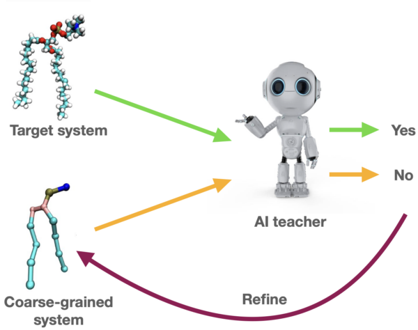
Fig: Interplay between coarse-grained model and AI teacher.
This iterative process is akin to a continuous loop of hypothesis and verification, where the CG model proposes a set of dynamics and the neural network validates them. Through this adversarial process, the CG model is constantly learning and adjusting. It refines its parameters to better mimic the real system’s behavior, enhancing its ability to predict new situations with greater accuracy.
This methodology that we are developing offers a new perspective on modeling the dynamics of biomolecular systems, showing instead of their direct application in scientific discovery, the AI models synergize with existing methods to embrace the application in challenging situations. With the support of AI and powerful computational resources, we are moving steadily toward precise and efficient digital simulations of living systems.
This work was supported by the Eric and Wendy Schmidt AI in Science Postdoctoral Fellowship, a program supported by Schmidt Sciences.
May 16, 2024

Expanding Our Vocabulary of Vision Using AI
Ramanujan Srinath, Eric and Wendy Schmidt AI in Science Postdoctoral Fellow

Figure 1. AI methods and models have enabled a huge leap in our understanding of how images are processed in the brain. We used to describe visual neurons as “edge detectors” and “face detectors”. Using deep neural networks, we have discovered that images like these (which really can’t be described with words) are richer models of single neurons in our visual system. I liken these AI-enabled descriptions of neural function, perhaps ironically, to a whole new kind of vocabulary that neuroscientists can now use to explain the visual system. (Images from various papers including a, b, c, d, e , f)
Our perception of the world is inexorably linked to the words we use to describe it. Our appreciation for and ability to discriminate between different
Our perception of the world is inexorably linked to the words we use to describe it. Our appreciation for and ability to discriminate between different colors or different artistic styles is markedly improved after we acquire the words to describe those colors or artworks. This is called linguistic relativity, and while specific examples might be controversial, it certainly has caught the eye of storytellers. In the book 1984, the authoritarian government introduced ‘Newspeak’ to inhibit people from being able to think critically about policy or oppression. And in Arrival, aliens introduce humans to their language to help the humans perceive time differently. In the real world, machine learning and AI methods developed less than a decade ago have introduced a new kind of vocabulary to the neuroscientific understanding of how we see and have had the same kind of revolutionary effect on the field.
Let’s rewind 50 years or so. Neurobiologists had figured out a lot about how neurons work: how they communicate with each other, the anatomy of the eye and various parts of the brain, and the effect of many drugs on the brain and behavior. But questions about how the brain receives inputs from the eye and produces percepts required a fundamental shift in our understanding of the visual system. Hubel and Wiesel initiated that shift with their discovery of neurons in the brain that are activated by elongated bars of light displayed on a screen. These neurons cared about the orientation of the bar and were dubbed “orientation tuned neurons” because, like you tune an FM radio to a channel frequency, you could tune the activity of the neuron with the orientation and the direction of the moving bar of light. And thus we have our first word — “orientation” — to describe a class of visually sensitive neurons. We can also say that “orientation tuning” is a “word model” of what this neuron does.

Figure 2. Oliver Selfridge, an AI pioneer, introduced the pandemonium model of visual pattern recognition in 1959 in which mental “demons” identify simple patterns and lines in the stimuli and shout them out. Cognitive demons listen to these shouts and match it to their more complex patterns. And at the very end, decision demons categorize what is being seen and decide how to interpret or act. This model in various evolved forms was the basis of visual cognitive and neuroscientific thought for decades. (Figure adapted from Lindsay and Norman, 1972)
Since then, neuroscientists have marched faithfully along the hierarchy of visually sensitive areas in the brain to find new kinds of neurons that are activated by different features displayed on the screen. For instance, you can imagine a neuron connected to two orientation tuned neurons to become an “angle” or “corner” neuron. You can put many of them together to form a “curvature” neuron. Instead of edges, you can have neurons sensitive to different “colors” and “textures.” Put all these together to form “object” or “face” or “tool” or “landscape” neurons. You can discover anatomical connections between the hierarchy of visual areas in the brain and come up with theories about how these neurons develop their sensitivities and what would happen if the inputs from the eyes were degraded somehow. If you tell a neuroscientist that a neuron in a specific part of the brain is orientation tuned, they can guess its provenance, development, anatomical connections with its inputs and outputs, the properties of the neurons in its neighborhood, and what would happen if you removed it from the circuit. We have been asking these questions and enriching our understanding of how we visually perceive for decades.
But there has always been a sword of Damocles hanging above our models of vision. Remember the “orientation” tuned neuron? That one was a bit of an exception, turns out*. As soon as you put two of these simple neurons together, the number of types of responses explode. Indeed, even Hubel and Wiesel thought it “unwise” to label neurons “curvature” or “corner” detectors because those monikers “neglect the importance of” the other properties of objects. They simply labeled them “simple”, “complex” or “hypercomplex” cells and described their responses in great detail while admitting that they were describing a subset of all types and that their descriptions were very likely impoverished. Because of this, none of our models were able to generate good predictions about how neurons would respond to photographs of natural scenes which have an intractably rich variety of visual features. Nevertheless, for fifty years, we have been using all these categorical words to describe the neurons that mediate our perception of the visual world, knowing full well that the categories are imperfect and their boundaries permeable.
*In fact, even those neurons aren’t exceptions and orientation tuning as a model is probably just as impoverished a model as any other.
About a decade ago, visual neuroscientific inquiry was introduced to a new kind of vocabulary, a new kind of model of a neuron. Neuroscientists discovered that deep convolutional neural networks that were trained to categorize images (like AlexNet) contained units that could model the responses of visual neurons better than any other model we had. Let’s unpack that.
A machine learning model was trained to bin images into categories like “German Shepard dog” or “table lamp” or “pizza.” It just so happens that the units of computation in that model (individual filters or combinations of filters) respond in similar ways to input images as the units of computation in our brains (individual neurons or combinations of neurons). Scientists could also invert this argument and test the validity of the model by generating images for which the models have specific predictions for neural activity. In other words, they could use the model to create an image that could activate a neuron in the brain more than any other image. So all you need to describe a visual neuron is this image generated by the best model of that neuron — the more like this image a random photograph was, the more the neuron would respond. Now, instead of saying a neuron was “orientation tuned,” you could provide either the deep network model that predicts its activity or an image that maximally drives the neuron.
These findings have moved the needle significantly for many visual neuroscientists. For some, these models are hypothesis generation machines — a good model can predict the responses of neurons in a variety of untested conditions like testing a deep network face neuron model on objects. For others, these models are edifices to be challenged — testing images for which the models have nonsensical predictions about how the brain extracts image information. And for still others, a deep network model of a neuron is a total replacement of the word models that came before it. For most, in the belabored metaphor introduced at the top of this article, these models and images have added a fundamentally new kind of vocabulary to how we describe visual neurons.
This raises deep questions about the goal of the visual neuroscientific enterprise. Are models of neurons that predict their responses to a very large, diverse set of images sufficient to understand visual perception? More fundamentally, what does it mean to “understand” vision? At the limit, if I could create a model that could precisely predict the responses of a visual neuron to every image, have we “understood” vision? Can we declare victory if we have a card catalog of images that maximally drive every single visual neuron in the brain?
Maybe a hint of an answer comes from Hubel and Wiesel themselves — “… it should perhaps be stressed that a proper understanding of the part played by any cell in a sensory system must depend not simply upon a description of the cell’s responses to sensory stimuli, but also on a knowledge of how the information it conveys is made use of at higher levels… How far such analysis can be carried is anyone’s guess, but it is clear that these transformations … go only a short way toward accounting for the perception of shapes encountered in everyday life.” Also, in the words of perhaps one of the leading philosophers of our time, ChatGPT:

Figure 3. Example of ChatGPT output.
I take inspiration from that challenge in my work as a Schmidt Sciences AI in Science Postdoctoral Fellow in the Department of Neurobiology. I am interested in how dimensions of visual information are extracted by the brain and then used to make decisions. In a recent study, we showed that the reason we can extract information about foreground objects while the background changes dramatically is that the visual information about the foreground and the background is represented orthogonally in the brain. In an upcoming manuscript, we demonstrate that visual neurons guide the extraction of information and the behavior based on that information by flexibly modifying their responses based on cognitive demands. We also discovered a possible mechanism by which these visual neurons could be doing that using simulations and AI methods. Stay tuned for an article about those results!
This work was supported by the Eric and Wendy Schmidt AI in Science Postdoctoral Fellowship, a program supported by Schmidt Sciences.
May 9, 2024

Teaching materials to adapt
Martin Falk, Eric and Wendy Schmidt AI in Science Postdoctoral Fellow
Considered as materials, biological systems are striking in their ability to perform many individually demanding tasks in contexts that can often change over time. One noticeable feature of biological materials is their adaptability, the ability of a material to switch between mutually incompatible functions with minimal changes. Consider the skin of a chameleon; with just a few changes to the structure of pigments in its cells, a chameleon’s skin is capable of becoming a totally different color. What sort of processes could create materials which could also rapidly switch function, like a chameleon’s skin?
It turns out that the two key ingredients for producing adaptability in biology are fluctuating environments and having many designs which achieve the same function. By continually forcing organisms to adapt to different stresses, evolution in fluctuating environments selects for the rare design solutions which can be rapidly switched, should the environment fluctuate again.

Caption: (left) We want to find networks which can easily switch between two different motions. (right) Alternating the design process for each motion results in networks which can easily switch between the two motions.
My collaborators and I have been thinking about how this intuition can be adapted not just for biological systems which evolve, but also for materials which we design. We designed an elastic network to exhibit an out-of-phase allosteric motion – that is, if you pinch the network on the bottom, it will spread apart on the top. We also made networks that have in-phase allosteric motion – pinching these networks on the bottom will result in the network also pinching in on the top. For both of these motions, there are many different network designs which will achieve the desired motion. However, if you compare two random networks, one for each motion, you will see that the networks chosen are very different. Such networks are not adaptable; it would take many changes to the network structure in order to switch from one network to the other.
Excitingly, we found that if you alternate back and forth between designing first for the out-of-phase motion and then for the in-phase motion, the elastic network solutions you find will look very similar to each other! Therefore, despite the fact that the out-of-phase motion and the in-phase motion are totally opposite types of motions, we found materials which can rapidly adapt between them. Furthermore, just as our intuition from biology suggests, these adaptable networks are much rarer, and hence we needed the alternating design process to find them.
We also tested our alternating design process in two other kinds of material systems: elastic networks created to have different bulk material properties, as opposed to motions, as well as polymers created to fold into different structures, like proteins. In each case, we found that alternating design goals resulted in adaptable materials. In the case of the polymers folding into different structures, we were also able to identify a physical principle underlying the existence of these adaptable materials – the physics of phase transitions, the same physics underlying the tempering of chocolate. Therefore, our method not only worked, but also helped us to better understand how materials can be made to adapt.
We’re excited by our alternating design procedure because it can be applied across a wide range of different materials, taking advantage of the unique aspects of each material in order to produce adaptability. In the future, we want to think about the implications of alternating design in artificial neural networks. Like our materials, artificial neural networks succeed because there are many different network configurations capable of fitting the data that the networks are trained on. However, neural networks are usually trained to perform a single (albeit complicated) task. Can we use inspiration from how nature adapts and changes to train artificial neural networks to have even more sophisticated properties?
This work was supported by the Eric and Wendy Schmidt AI in Science Postdoctoral Fellowship, a program supported by Schmidt Sciences.
May 2, 2024

From Protein Structures to Clean Energy Materials to Cancer Therapies: Using AI to Understand and Exploit X-ray Damage Effects
Adam Fouda, Eric and Wendy Schmidt AI in Science Postdoctoral Fellow
X-rays are not just the workhorse for imaging bone structures in our bodies, they are also the workhorse of materials characterization techniques across the biological, chemical and physical sciences. However, the absorption of x-rays by atoms creates unstable states which undergo complex decay process that can damage the structures during their characterization.
Interestingly though, this x-ray damage process is not all bad. In some cases, detecting it can itself be a powerful characterization tool; and furthermore, the effect is now being explored in novel cancer therapies that selectively target tumor cells. The physics underlying damage effect is described by quantum mechanics (the theory describing the behavior of atoms and electrons), this limits its effective simulation in complex real-world systems. However, the opportunity for AI accelerated predictions of more complex systems has emerged through the development of accurate quantum mechanical methods for generating small molecule datasets and the availability of benchmark experiments.
X-rays can characterize the arrangement of atoms forming the shape of complex materials, such as proteins or nanoparticle catalysts through x-ray scattering techniques. They can also interrogate the arrangement of electrons forming chemical bonds around a selected atom site through x-ray spectroscopy, which involves the absorption of x-rays by the atoms. Whilst the dosage of x-rays safely used in everyday medical applications is relatively low; effectively interrogating the microscopic world of atoms requires exceptionally bright x-ray sources generated at large-scale facilities with circular particle accelerators called synchrotrons. Synchrotrons pass electrons through a sequence of magnets at almost the speed of light, where they can then produce x-rays 10 billion times brighter than the sun. Researchers utilize the powerful characterization properties of the bright x-rays on subjects ranging from combustion engines, batteries, protein structures, cancer treatments and advanced research materials.
X-ray damage effects happen when x-ray absorption interferes with x-ray scattering measurements. For example, in proteins that contain metal atoms, the absorption of metal atoms by the x-rays dominates the interaction during the scattering measurement. Consequently, almost all such protein structures reported in the protein databank are compromised. This happens because the x-ray absorption removes the electrons most tightly bound to the atoms nucleus. This creates an unstable state that collapses by a complicated decay process which ejects multiple electrons from the atom. The removal of negatively charged electrons leaves a positively charged environment about the metal atom which changes the protein structure during the x-ray scattering characterization.
However, this x-ray damage process can in-fact be utilized. Detecting these ejected electrons provides a complex but detailed characterization of the electronic arrangements about the absorbing atom site, which offers the opportunity for more sensitive x-ray spectroscopy methods. This is because the ejected electrons are not tightly bound to the nucleus and are more involved with the bonding to the neighboring atoms. Another useful property of the ejected electrons is that they can have relatively low energies compared to fluorescence decay and the nuclear decay of radioactive atoms. The low energy ejected electrons have short travel distances in aqueous environments because they are likely to ionize nearby water molecules. This makes them effective at characterizing the structure of a materials surface in an aqueous solution. This has successfully been applied to characterizing the differences in water molecule arrangements at the material surface and bulk solution in a battery cell system.
The short travel distances in aqueous environments has applications beyond materials characterization. Novel radionucleotide cancer therapies also exploit this effect. Once a radionucleotide atom in a molecule undergoes a nuclear decay process, a tightly bound electron is also lost from it. This mimics x-ray absorption and initiates the same decay cascade process. Near a tumor cell, the low energy electrons ejected from the radionucleotide and neighboring atoms can effectively damage the tumor whilst causing minimal damage to the surrounding tissue. This treatment is therefore less damaging to the patient than traditional cancer therapies using the high energy alpha and beta decays.
Despite all these advantages, it’s hard to simulate the decay process as it relies on quantum mechanics. Furthermore, the number of possible decay channels scales exponentially with the size of the system and simulations are thus restricted to atoms, small molecules, and simplistic aqueous environments.
However, reliable AI predictions of larger systems are now possible through recent developments in accurate and efficient methods for small (5-10 atoms) organic molecules, and the availability of benchmark experimental data on these systems and more complex ones. We are developing a deep neural network that inputs information of the atomic placements about the absorbing atom site and outputs the decay signal. The input only requires the knowledge of the molecular geometry, and the trained model will therefore bypass the need for further quantum mechanics calculations.

Fig: The neural network will be trained on a dataset generated by validated quantum mechanics methods on small molecules. The model will then be used to predict the x-ray damage effect in more complex systems.
Because the decay of each individual absorbing atom is mostly affected by its adjacent atoms, we believe our trained model will accurately predict the decay of organic molecules too large for a quantum mechanics simulation. Our model will be trained across thousands of different atomic environments across a set of mid-size organic molecules. Therefore, the model should be able to combine any number of different local atomic environments together to generate the decay signals of much larger systems. Successfully demonstrating this will open a new AI research direction, where the continual development of dataset diversity, model architecture and experimental collaboration will pave the way for AI to drive understanding and exploit the role of this x-ray damage effect in important real-world applications.
This work was supported by the Eric and Wendy Schmidt AI in Science Postdoctoral Fellowship, a Program supported by Schmidt Sciences, LLC.
April 24, 2024

Towards New Physics at Future Colliders: Machine Learning Optimized Detector and Accelerator Design
Anthony Badea, Eric and Wendy Schmidt AI in Science Postdoctoral Fellow
We are in an exciting and challenging era of fundamental physics. Following the discovery of the Higgs boson at CERN’s Large Hadron Collider (LHC), there have been 10 years of searches for new physics without discovery. The LHC, shown below, collides protons at nearly the speed of light to convert large quantities of energy to exotic forms of matter via the energy-mass relationship E=mc2. The goal of our searches is to discover new particles which could answer some of the universe’s most fundamental questions. What role does the Higgs play in the origin and evolution of the Universe? What is the nature of dark matter? Why is there more matter than antimatter in the universe? Given the absence of new particles, the field is devising new methods, technologies, and theories. Some of the most exciting work is towards building more powerful colliders. In this work, an emerging theme is the use of machine learning (ML) to guide detector and accelerator designs.

Figure 1: Aerial view of the 27-kilometer-long Large Hadron Collider (LHC) located on the border of France and Switzerland near Geneva. The LHC collides particles at nearly the speed of light to study the universe in a controlled experimental facility. The Higgs boson was discovered with the LHC in 2012. Image credit to ESO Supernova.
The goal of building new colliders is to precisely measure known parameters and attempt to directly produce new particles. As of 2024, the most promising designs for future colliders are the Future Circular Collider (FCC), Circular Electron Positron Collider (CEPC), International Linear Collider (ILC), and Muon Collider (MuC). The main difference between the proposals is the type of colliding particles (electrons/positrons, muons/anti-muons, protons-protons), the shape (circular/linear), the collision energy (hundreds vs. thousands of gigaelectronvolts), and the collider size (10 – 100 km). A comparison between the current LHC and proposed future colliders is shown below.
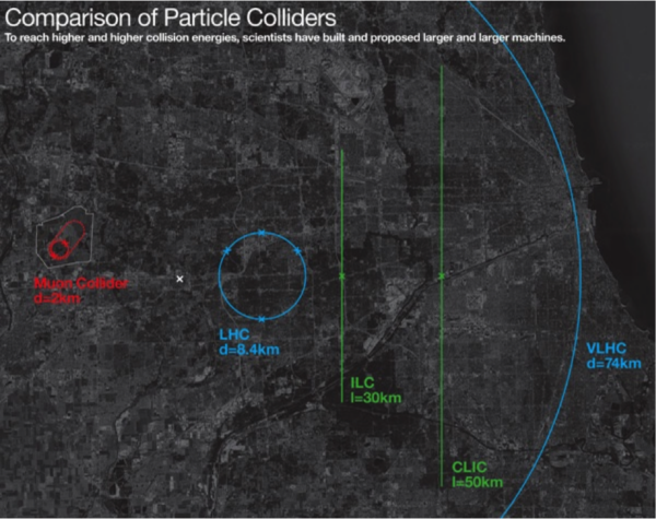
Figure 2: Size comparison between the current LHC and proposed future colliders: Muon Collider (red), LHC (light blue), International Linear Collider (green), and Very Large Hadron Collider (outmost light blue labeled as VLHC). Note the VLHC was a similar proposal but is roughly twice as large as the Future Circular Collider. Image credit Fermilab.
Designing the accelerator and detector complexes for future colliders is a challenging task. The design involves detailed simulations of theoretical models and particle interactions with matter. Often, these simulations are computationally expensive, which constrains the possible design space. There is ongoing work to overcome this computational challenge by applying advances in surrogate modeling and Bayesian optimization. Surrogate modeling is a technique for creating a fast approximate simulation of an expensive, slow simulation, increasingly using neural networks. Bayesian optimization is a technique to optimize black box functions without assuming any functional forms. The combination of these approaches can reduce computing expenses considerably.
An example of ML guided optimization is ongoing for one of the outstanding challenges for a MuC. A MuC is an exciting future collider proposal that would be able to reach high energies in a significantly smaller circumference ring than other options. To create this machine, we must produce, accelerate, and collide muons before they decay. A muon is a particle similar to the electron but around 200 times heavier. The most promising avenue for this monumental challenge starts by hitting a powerful proton beam on a fixed target to produce pions, which then decay into muons. The resulting cloud of muons is roughly the size of a basketball and needs to be cooled into a 25µm size beam within a few microseconds. Once cooled, the beam can be rapidly accelerated and brought to collide. The ability to produce compact muon beams is the missing technology for a muon collider. Previously proposed cooling methods did not meet physics needs and relied on ultra-powerful magnets beyond existing technology. There are alternative designs that could remedy the need for powerful magnets, but optimization of the designs is a significant hurdle to assessing their viability.
In a growing partnership between Fermilab and UChicago, we are studying how to optimize a muon-cooling device with hundreds of intertwined parameters. Each optimization step will require evaluating time and resource intensive simulations, constraining design possibilities. So, we are attempting to build surrogates of the cooling simulations and apply Bayesian optimization on the full design landscape. There have been preliminary results by researchers in Europe that show this approach has potential, but more work is needed.
To make progress on this problem, we are starting simple – trying to reproduce previous results from classical optimization methods. Led by UChicago undergraduates Daniel Fu and Ryan Michaud, we are performing bayesian optimization using gaussian processes. This does not include any neural networks but helps build our intuition for the optimization landscape and mechanics of the problem. The first step of this process is determining if the expensive simulation can be approximated by a gaussian process to produce a fast surrogate. If it can be then the optimization can proceed. If not then we’ll need to deploy a more complex model like a neural network. We hope to have preliminary results by the summer ‘24 and contribute to the upcoming European strategy update for particle physics.
This work was supported by the Eric and Wendy Schmidt AI in Science Postdoctoral Fellowship, a program supported by Schmidt Sciences.
April 18, 2024
Uncovering Patterns in Structure for Voltage Sensing Membrane Proteins with Machine Learning
Aditya Nandy, Eric and Wendy Schmidt AI in Science Postdoctoral Fellow
How do organisms react to external stimuli? The molecular details of this puzzle remain unsolved.
Humans, in particular, are multi-scale organisms. Various biological systems (i.e. the respiratory system, digestive system, cardiovascular system, endocrine system, etc.) comprise the human body. Within each of these systems, there are organs, which are made of tissues. Each tissue is then made of cells. Within cells, there are smaller pieces of machinery known as organelles. Cells and organelles are composed of a variety of proteins and lipids. In particular, proteins that are embedded in lipids (as opposed to floating within the cell) are known as membrane proteins.
Although there are clear differences between organisms (i.e. bacteria, humans, and mice) at the cellular and atomic scales, the protein machinery looks very similar. Indeed, challenges in predicting protein structure led to the breakthrough of AlphaFold, enabling scientists to make predictions on protein structure given a primary sequence of amino acids (the building blocks of proteins). Cells and organelles across different organisms sense stimuli such as touch, heat, and voltage with a specific type of protein called a membrane protein. These membrane proteins are usually embedded on the membrane that defines the “inside” and “outside” of a cell or an organelle, and thus are responsible for sensing. Despite advances in protein structure prediction with AlphaFold, challenges remain for predicting the structures of membrane proteins. We can utilize existing experimental structures, however, to try and decipher patterns for voltage sensing.
Voltage Sensing Proteins
Voltage sensing membrane proteins are specialized molecular entities found in the cell membranes of various organisms, ranging from bacteria to humans. These remarkable proteins play a pivotal role in cellular function by detecting and responding to changes in the electrical potential across the cell membrane. Through their sophisticated structure and mechanisms, voltage sensing membrane proteins enable cells to perceive, process, and transmit electrical signals essential for vital physiological processes such as neuronal communication (i.e. passing action potentials), muscle contraction, and cardiac rhythm regulation. For instance, neurons have voltage-gated ion channels – channels that open and allow the flux of ions into the cell to produce electrical signals.
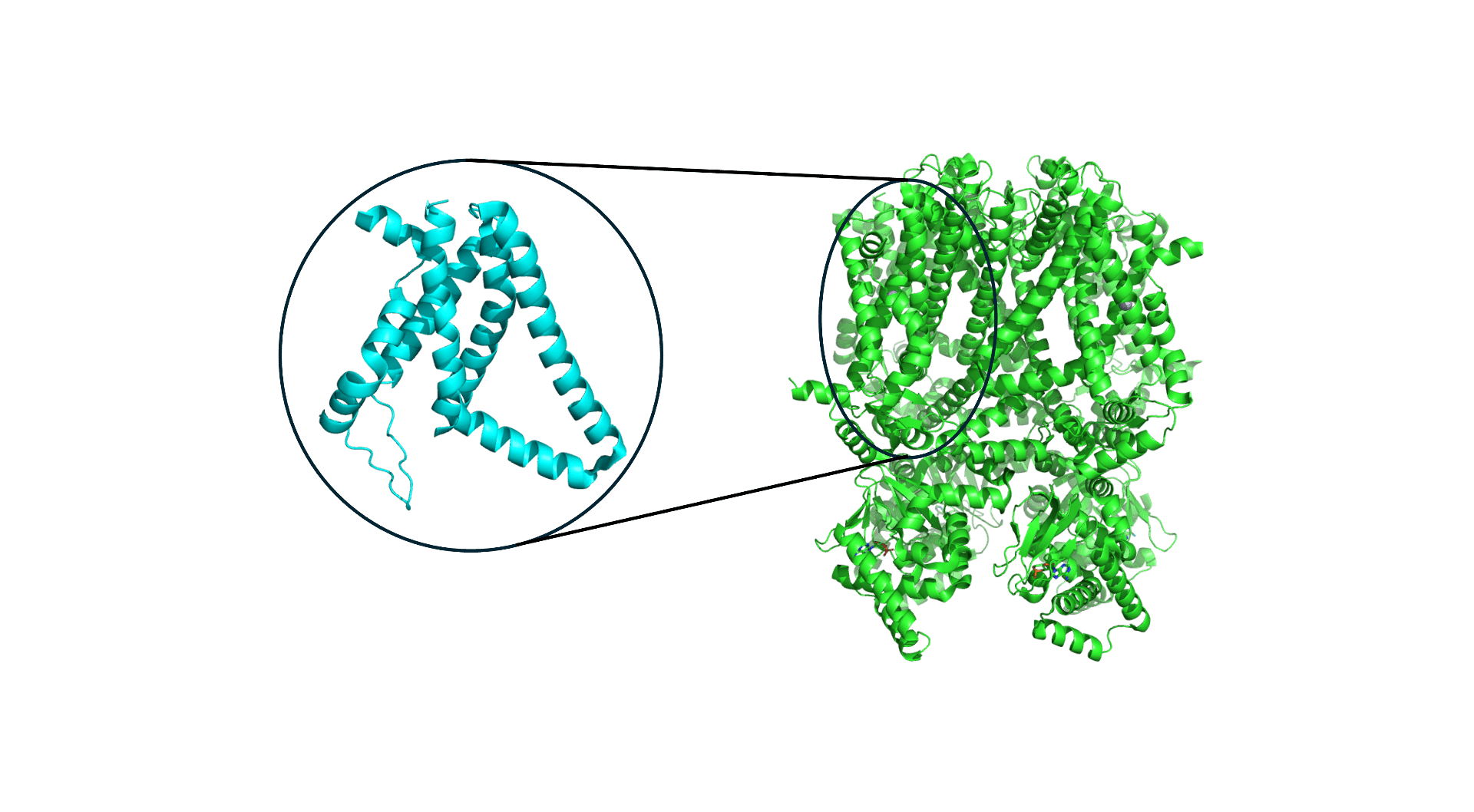
Despite the complexity of voltage sensing proteins that are able to sense different voltages with high sensitivity, the biology of voltage sensors is highly modular. Proteins that respond to voltage typically have what is known as a “voltage sensing domain,” or VSD. The VSD is usually coupled to a larger module that is responsible for function. For instance, in a voltage-gated ion channel, the ion channel itself is coupled to one or more VSDs that enable it to behave in a voltage-sensitive way. The modular nature of the VSD, which is nearly always a 4-helix bundle, enables comparison across VSDs from different proteins (and organisms!) using machine learning. Over the full protein data bank (PDB) where protein structures are deposited by experimental structural biologists, we can extract thousands of VSDs from various proteins.
Figure 1. A typical voltage sensor (left) for a membrane protein (right) that has multiple voltage sensing domains.
Analogy to Modified NIST (MNIST) Digit Dataset
At its root, we would like to determine any patterns between voltage sensors that may have similar function, turning the problem into one of “pattern recognition” that can be tackled with machine learning. Analogous pattern recognition problems have been carried out by computer scientists for decades. The MNIST data set is a classic task in machine learning for classifying hand-written digits. The key concept in classifying MNIST digits is that each digit has a set of characteristics, or “features,” that underlies its membership to a certain label (in this case, 1 through 9). Humans can identify these digits, but a machine learning model must pick out the key similarities and differences between these digits to separate them.
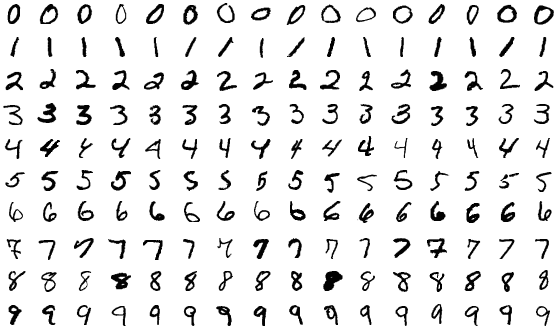
Figure 2. Digits from MNIST (left, figure adapted from Wikipedia). Digits are hand-written. Each row represents a category of digits.
In a similar vein, VSDs must have underlying features and characteristics that make them uniquely sensitive to different voltages. One key difference that makes working with scientific data more challenging than MNIST is that we do not always have labels. Or more specifically, we do not know the sensitivity of the voltage sensor unless a functional study has been carried out.
The Excitement
Using machine learning to fingerprint and cluster VSDs represents an opportunity to move beyond sequence-to-structure prediction, like AlphaFold, and on to structure-to-function analysis. Through analyses on structural similarities and differences, we may be able to discern the molecular basis for voltage sensitivity and the key structural features that are essential for a protein to respond to voltage. Understanding this response to voltage can help us understand how the molecular machinery of the body behaves under native and diseased conditions.
Together with the Vaikuntanathan, Roux, and Perozo laboratories and the newly formed Center for Mechanical Excitability at the University of Chicago, I continue to investigate voltage-sensitive proteins to understand how they underlie how cells respond to stimuli.
This work was supported by the Eric and Wendy Schmidt AI in Science Postdoctoral Fellowship, a program supported by Schmidt Sciences.
April 11, 2024

Finding the likely causes when potential explanatory factors look alike
William Denault, Eric and Wendy Schmidt AI in Science Postdoctoral Fellow
Suppose you are a scientist interested in investigating if there is a link between exposure to car pollutants during pregnancy and the amount of brain white matter at birth. A starting hypothesis you would like to test could be: is an increase of a specific pollutant associated with a reduction (or increase) of white matter in newborns? A typical study to test this hypothesis would involve recruiting pregnant women, measuring the average amount of pollutants they are exposed to throughout their pregnancy, and measuring the newborn’s proportion of white matter, which is a measure of connectivity. After the collection, the data analysis would involve assessing if at least one of the car pollutants is correlated with the newborn’s brain measurements. It is now well established that exposure to car pollutants during pregnancy is associated with reduced white matter proportion in newborns. A natural follow-up question would be among all these car pollutants which is likely to cause a reduction in white matter? That is when things become more tricky.
Because cars tend to produce the same amount of each pollutant (or at least the proportion of pollutants they emit is somewhat constant), we observe little variation in car pollutant proportion over time in a given city. It would be even worse if we only studied women from the same neighborhood and recruited them during a similar period of time (as we expect the car pollutants to be quite homogeneous within a small area). The main difficulty in trying to corner a potential cause among correlated potential causes is that if pollutant A ( e.g., Carbon Monoxide CO) affects the newborn white matter but pollutant B (e.g., Carbon Dioxide C2O) is often producing along with pollutant A, it is likely that both pollutants will be correlated with newborn white matter proportion.
Correlation has been a primary subject of interest since the early days of statistics. While correlation is often a quantity of inferential interest (e.g., predicting house price given its surface), in some cases, it can plague an analysis as it is hard to distinguish between potential causes that are correlated (as described above).
Assume now that exactly two pollutants among four that are affecting newborn white matter. Pollutants 1 and 3, say — and that these two pollutants are each completely correlated with another non-effect pollutant, say pollutants 1 and 2 are perfectly correlated and pollutants 2 and 4. Here, because the pollutants are completely correlated with a non-effect pollutant, it is impossible to confidently select the correct pollutants that are causing health problems. However, it should be possible to conclude that there are (at least) two pollutants that affect white matter, for the first pollutant that affects white matter it is whether (pollutant 1 or pollutant 2), for the first pollutant that affects white matter it is whether (pollutant 3 or pollutant 4).
This kind of statement (pollutant 3 or pollutant 4) is called credible sets in the statistical genetic literature. Credible sets are generally defined as follows. A credible set is a subset of the variables that have at least 95% to contain at least one causal variable. In our example, the pollutants are the variables. Inferring credible sets is referred to as fine mapping.
Until recently, most of the statistical approaches were working well for computing credible sets in the case that exactly one pollutant affects newborn white matter. Recent efforts led by the Stephens’ lab and other groups suggest enhancing previous models by simply iterating them through the data multiple times. For example, suppose I have made an initial guess for the credible sets for the first effect pollutant. Now, I can remove the effect of the pollutant from my data and guess the credible sets for the second effect. Once this is done, we can refine our guess for the first pollutant by removing the effect of the second credible set from the data and continuing to repeat this procedure until convergence.
The example we presented above is quite simple as a maximum of a hundred pollutants and derivatives are being studied, and they can be potentially tested one by one in a lab using mice. The problem becomes much harder in genetics, where scientists try to understand the role of hundreds of thousands of variants on molecular regulation. And in fact, genetic variants tend to be much more correlated than car pollutants. And this complexity increases as we try to understand more complex traits. For example, instead of just trying to see if exposure to car pollutants affects the white matter at birth, we could see if that affects the proportion of white matter throughout childhood.
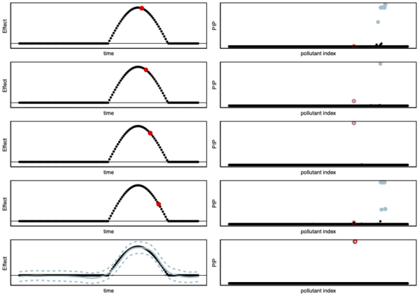
Illustration of our new fin-mapping method (fSuSiE) for fine-mapping dynamic/temporally structured traits. In this example, we consider a pollutant that decreases the amount of white matter during a certain duration during childhood. This effect is displayed in the left column. We are trying to corner the causal pollutant among 100 candidates. The index of the causal pollutant is displayed in red on the right column, and the index of the other candidate pollutants is displayed in black. One approach might be to fine-map each time point independently, for example, using previous fine-mapping methods like SuSiE. In this example, we run SuSiE at each time point to identify the causal pollutant. SuSiE detected the effect of pollutants at only 4 time points (first top four panels). The different 95% credible sets (blue circles) are displayed on the right-hand side. We observe that the PIPs (probabilities of being the causal SNP) are different at each time point. On the other hand, fSuSiE identifies the causal pollutant in a credible set containing a single pollutant (lowest panel). Additionally, fSuSiE estimates the effect of the causal pollutant. The black line is the true effect; the solid blue line is the posterior mean estimate; and the dashed blue lines give the 95% posterior credible bands.
Our current work is generalizing the iterative procedure described here to a more complex model. One of the main difficulties is to find a good trade-off between model complexity and computational efficiency. More complex models capture more subtle variation in the data but are more costly to estimate. We use ideas from signal processing methods (wavelet) to perform fast iterative procedures to corner genetic variants (or car pollutants) that affect dynamic or spatially structured traits (e.g., white matter development throughout childhood or DNA methylation). We present some of the advantages of our new work in Figure 1.
Coming back to our earlier example where pollutants 1 and 3 affect white matter. The main problem with fine-mapping pollutants that affect temporally-structured traits is that standard fine-mapping may suggest that pollutant 1 affects white matter proportion at birth but then may suggest that pollutant 2 affects white matter at three months. Thus leading to inconsistent results throughout childhood. Using a more advanced model that can look at each child’s trajectory (instead of at each time point separately as normally done) allows for more consistent and interpretable results. We illustrate this advantage in Figure 1.
This work was supported by the Eric and Wendy Schmidt AI in Science Postdoctoral Fellowship, a program supported by Schmidt Sciences.
April 4, 2024

Leveraging machine learning to uncover the lives and deaths of massive stars using gravitational waves
Thomas Callister, Eric and Wendy Schmidt AI in Science Postdoctoral Fellow
For all of human history, astronomy has consisted of the study of light. Different wavelengths of light are detected in different ways and used for different purposes. Traditional telescopes collect and focus optical light (the same wavelengths seen by the eye) in order to view distant stars and galaxies. Large radio dishes capture the much lower frequency radio waves that comprise the Cosmic Microwave Background, a baby picture of the early Universe. And x-ray telescopes in orbit around the Earth catch bursts of high-energy light from all manner of explosions throughout the Universe. Whatever the wavelength, though, these are all differential realizations of the same physical phenomenon: ripples in the electromagnetic field, a.k.a. electromagnetic waves, a.k.a. light.
Humanity’s astronomical toolkit categorically expanded in September 2015, with the first detection of a new kind of astronomical phenomenon: a gravitational wave. Gravitational waves are exactly what they sound like: a ripple in gravity. The new ability to detect and study these gravitational waves offers an entirely new means of studying the Universe around us, one that has allowed us to study never before seen objects in uncharted regions of the cosmos. I am one of two Eric and Wendy Schmidt AI in Science Postdoctoral Fellows (along with Colm Talbot) who study gravitational waves. I therefore want to broadly introduce this topic — what gravitational waves are and how they are detected — in order to set the stage for future posts exploring gravitational-wave data analysis and the opportunities afforded by machine learning.
If you have spent any time watching the History Channel or reading popular science articles, you have probably encountered the idea of gravity as curvature. Today, physicists understand the nature of gravity via Einstein’s General Theory of Relativity, which describes gravity not as an active force that grabs and pulls objects, but as the passive curvature or warping of space and time (together known as spacetime) by matter. The Earth, for example, is not kept in its orbit via a force exerted by the Sun. Instead, the Sun curves the surrounding fabric of spacetime, and the Earth’s motion along this curved surface inscribes a circle, just like a marble rolling on some curved tabletop. This arrangement is often summarized as follows: “Matter tells spacetime how to bend, spacetime tells matter how to move.”
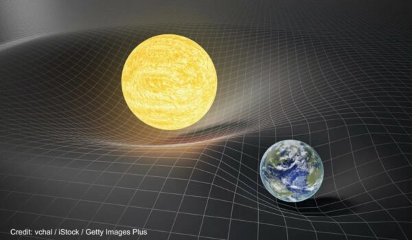
Gravity and general theory of relativity concept. Earth and Sun on distorted spacetime. 3D rendered illustration.
With this analogy in mind, now imagine doing something really catastrophic: crash two stars together; let the Sun explode; initiate the birth of a new Universe in a Big Bang. Intuition suggests that the fabric of spacetime would not go undisturbed by these events, but would bend and vibrate and twist in response. This intuition is correct. These kinds of events indeed generate waves in spacetime, and are what we call gravitational waves. Strictly speaking, almost any matter in motion can generate gravitational waves. The Earth generates gravitational waves as it orbits the Sun. You generate gravitational waves any time you move. In practice, however, only the most violent and extreme events in the Universe produce gravitational waves that are remotely noticeable, and even these end up being extraordinarily weak. To explain what exactly I mean “extraordinarily weak,” I first have to tell you what gravitational waves do.
I introduced gravitational waves via an analogy to light; the latter is a ripple in the electromagnetic field and the former a ripple in the gravitational field. This description, though hopefully intuitive, masks a fundamental peculiarity of gravitational waves. All other waves — light, sound waves, water waves, etc. — are phenomena that necessarily move inside of space and time (it would not make sense for anything to exist outside space and time!). Gravitational waves, though, are ripples of space and time. There is no static frame of reference with which to view gravitational waves; gravitational waves manifest as perturbations to the frame itself.
What does this mean in practice? The physical effect of a gravitational wave is to modulate the distances between objects. Imagine two astronauts floating freely in space. A passing gravitational wave will stretch and shrink the distance between them. Critically, this occurs not because the astronauts move (they remain motionless), but because the space itself between them literally grows and shrinks (think of Doctor Who’s Tardis, wizarding world tents in Harry Potter, the House of Leaves’s House of Leaves). The strength of a gravitational wave, called the gravitational-wave strain and denoted h, describes this change in distance induced between two objects, ΔL, relative to their starting distance L:
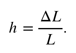
This change in length is exactly how gravitational waves are detected. Gravitational waves are detected by a network of instruments across the globe, all of which use lasers to very precisely monitor the distances between mirrors separated by several kilometers. These mirrors are exquisitely isolated from the environment; to detect a gravitational wave, you must be utterly confident that the distances between your mirrors fluctuated due to a passing ripple in spacetime and not because of minuscule disturbances due to a car driving by, Earth’s seismic activity, ocean waves hitting the coast hundreds of miles away, etc.

Credit: NSF
What kinds of events can we observe via gravitational waves, utilizing these detectors? Consider an object of mass M moving at speed v some distance D away. The gravitational wave strain you experience from this object is, to an order of magnitude,
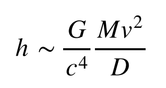
Here, I’ve used two additional symbols. The quantity ![]() is Newton’s gravitational constant and
is Newton’s gravitational constant and ![]() is the speed of light. Note that G is a very small number and c a very large number, so the ratio
is the speed of light. Note that G is a very small number and c a very large number, so the ratio ![]() in the equation above is extremely small, working out to about
in the equation above is extremely small, working out to about ![]() ! The extraordinary smallness of this number means that gravitational waves produced by everyday objects are so infinitesimal as to be effectively non-existent. Consider someone waving their arms (with, say mass M ∼ 10 kg at speed
! The extraordinary smallness of this number means that gravitational waves produced by everyday objects are so infinitesimal as to be effectively non-existent. Consider someone waving their arms (with, say mass M ∼ 10 kg at speed ![]() ) at a distance of one meter away from you. Plugging these numbers in above, we find that you would experience a gravitational-wave strain of only h ∼ 10^−44.
) at a distance of one meter away from you. Plugging these numbers in above, we find that you would experience a gravitational-wave strain of only h ∼ 10^−44.
The important takeaway is that only the most massive and fastest-moving objects in the Universe will generate physically observable gravitational waves. One example of a massive and fast-moving system: a collision between two black holes. The Universe is filled with black holes, and sometimes pairs of these black holes succeed in finding each other and forming an orbiting binary. Over time, as these black holes emit gravitational waves, they lose energy and sink deeper and deeper in one another’s gravitational potential. As they sink closer together, the black holes move ever faster, in turn generating stronger gravitational-wave emission and hastening their progress in an accelerating feedback loop. Eventually, the black holes will slam together at very nearly the speed of light. This entire process is called a binary black hole merger. How strong are the final gravitational waves from these black hole mergers? Let’s plug some numbers into our equation above. Assume that the black holes are ten times the mass of our sun, M ∼ 2 × 10^31 kg, that they are moving at the speed of light, v ∼ c, and that they are a Gigaparsec (i.e. a few billion light years) away, D ∼ 3 × 10^25 m. The resulting gravitational-wave strain at Earth is approximately h ∼ 10^−22.
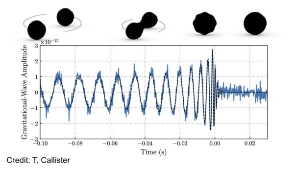
A binary black hole merger is just about the most massive and fastest moving system the Universe can provide us. And yet the gravitational waves it generates are still astonishingly small. To successfully measure waves of this size, gravitational-wave detectors have to track changes of size ΔL ∼ 10^−19 m in the distances between their mirrors. This is a distance one billion times smaller than the size of an atom. It is equivalent to measuring the distance to the nearest star to less than the width of a human hair. And although this sounds like an impossible task (and indeed was believed to be so for almost a century), decades of technological and scientific advancements have made it a reality. In September 2015, the gravitational-wave signal from a merging binary black hole a billion light years away was detected by the Advanced LIGO experiment, initiating the field of observational gravitational-wave astronomy.
We now live in a world in which gravitational-wave detection is a regular phenomenon. To date, about 150 gravitational-wave events have been witnessed. Most of these are from black hole collisions, and a handful involve the collisions of another class of object called a neutron star. How do we know the identities of these gravitational wave sources? And how does this knowledge help us study the Universe around us? (And where does machine learning come in??). Stay tuned to find out!
This work was supported by the Eric and Wendy Schmidt AI in Science Postdoctoral Fellowship, a program supported by Schmidt Sciences.
Mar 28, 2024
Leveraging machine learning to uncover the lives and deaths of massive stars using gravitational waves
Colm Talbot, Eric and Wendy Schmidt AI in Science Postdoctoral Fellow
Observations of merging binary black hole systems allow us to probe the behavior of matter under extreme temperatures and pressures, the cosmic expansion rate of the Universe, and the fundamental nature of gravity. The precision with which we can extract this information is limited by the number of observed sources; the more systems we observe, the more we can learn about astrophysics and cosmology. However, as the precision of our measurements increases it becomes increasingly important to interrogate sources of bias intrinsic to our analysis methods. Given the number of sources we expect to observe in the coming years, we will need radically new analysis methods to avoid becoming dominated by sources of systematic bias. By combining physical knowledge of the observed systems and AI methods, we can overcome these challenges and face the oncoming tide of observations.
A New Window on the Universe
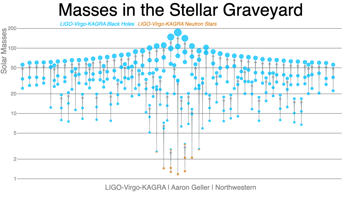
In September 2015, a new field of astronomy was born with the observation of gravitational waves from the collision of two black holes over a billion light years away by the twin LIGO detectors. In the intervening years, the LIGO detectors have been joined by the Virgo detector and similar signals have been observed from over 100 additional merging binaries. Despite this large and growing number of observations, many more signals are not resolvable by current detectors due to observational selection bias. An example of this selection bias is that more massive binaries radiate more than less massive binaries and so are observable at greater distances. Over the next decade, upgrades to existing instruments will increase our sensitivity and increase the observed catalog to many hundreds by the end of the decade. In addition, the planned next generation of detectors is expected to observe every binary black hole merger in the Universe, accumulating a new binary every few minutes.
Each of these mergers is the end of an evolutionary path from pairs of stars initially more tens of times massive than the Sun. Over their lives, these stars passed through a complex series of evolutionary phases and interactions with their companion star. This path includes extended periods of steady mass loss during the lifetime of the star, dramatic mass loss during a supernova explosion, and mass transfer between the two stars. Each of these effects is determined by currently unknown physics. Understanding the physical processes governing this evolutionary path is a key goal of gravitational-wave astronomy.
From Data to Astrophysics
Extracting this information requires performing a simultaneous analysis of all of the observed signals while accounting for the observation bias. Individual events are characterized by assuming that the instrumental noise around the time of the merger is well understood. The observation bias is characterized by adding simulated signals to the observed data and counting what fraction of these signals are recovered. In practice, the population analysis is performed using a multi-stage framework where the individual observations and the observation bias are analyzed with an initial simple model and then combined using physically-motivated models.
Using this approach we have learned that:
- black holes between twenty and a hundred times the mass of the Sun exist and merge; a previously unobserved population.
- there is an excess of black holes approximately 35 times the mass of the Sun implying there is a characteristic mass scale to the processes of stellar evolution.
- most merging black holes rotate slowly, in contrast to black holes observed in the Milky Way.
Growing Pains
Previous research has shown that AI methods can solve gravitational-wave data analysis problems, in some cases far more efficiently than classical methods. However, these methods also struggle to deal with the large volume of data that will be available in the coming years. As a Schmidt fellow, I am working to combine theoretical knowledge about the signals we observe with simulation-based inference methods to overcome this limitation and allow us to leverage the growing catalog of binary black hole mergers fully.
For example, while the statistical uncertainty in our inference decreases as the catalog grows, the systematic error intrinsic to our analysis method grows approximately quadratically with the size of the observed population. This systematic error is driven by the method used to account for the observational bias. In previous work, I demonstrated that by reformulating our analysis as a density estimation problem we can reduce this systematic error, however, this is simply a band-aid and not a full solution.
I am currently working on using approximate Bayesian computation to analyze large sets of observations in a way that is less susceptible to systematic error. An open question in how to perform such analyses is how to efficiently represent the large volume of observed data. I am exploring how we can use theoretically motivated pre-processing stages to avoid the need for large embedding networks that are traditionally used. By combining this theoretical understanding of the problem with AI methods I hope to extract astrophysical insights from gravitational-wave observations with both more robustness and reduced computational cost.
This work was supported by the Eric and Wendy Schmidt AI in Science Postdoctoral Fellowship, a program supported by Schmidt Sciences.
Mar 21, 2024

Spatial Immunity: A new perspective enabled by computer vision
Madeleine Torcasso, Eric and Wendy Schmidt AI in Science Postdoctoral Fellow
Our immune systems are complex and dynamic systems that help us survive when something goes wrong. Our bodies have developed little cellular armies that can take on all kinds of foes; they help to heal wounds, fight foreign invaders – like the common cold or COVID-19, and even battle cancer. There are many cell types that make up our immune systems, each having their own specialty. Some cells survey their native tissues, waiting for something insidious to come along. Other cells wait for the signal to build up their army – or proliferate – and mount an attack on that suspicious object. There are message-passing cells, killer cells, cells that act as weapon (or antibody) factories, cells that clean up the aftermath of an attack, and cells that keep the memory of the invader in case it’s ever seen again. A well-functioning immune system helps us to lead functional, long lives.
However, our immune systems are not always well-oiled machines. Autoimmune conditions are disorders where the immune system starts to attack normal, otherwise healthy tissue. These conditions can affect tissues and organs from any part of the body, ranging from rheumatoid arthritis, which affects the tissue in small joints; to multiple sclerosis, which affects the protective covering of nerves; to type 1 diabetes, which affects the insulin-producing cells in the pancreas. These conditions can all make everyday activities difficult, and even become life-threatening. In general, scientists understand the immune cell “major players” in many of these conditions, but sometimes these findings don’t translate effectively to patient care.
In patients diagnosed with lupus nephritis (an autoimmune condition that affects the kidneys), only about 15-20% of patients that are treated with existing therapies will respond to those therapies. And not responding to those therapies can have dire consequences – either a lifetime on dialysis or getting on a waitlist to receive a life-saving kidney transplant.
To effectively treat these conditions, we must first better understand them. New methods for imaging immune cells in their native tissue are helping us to uncover the differences between patients who do and do not respond to the current standard of care. Until recently, we have studied immune cells by taking them out of the affected tissue and testing them. Using these new imaging methods, we can now look at the diverse set of soldiers in these dysfunctional cellular armies while their “formations” are still intact. To do this, a small piece of tissue is taken from the affected organ and imaged with up to 60 different cell-tagging molecules. The resulting images are rich and complex – so much so that a human cannot easily interpret them. This is where artificial intelligence (AI), and more specifically computer vision, saves the day. We train a specific type of AI algorithm called a convolutional neural network (CNN) to find the tens of thousands of cells in the image of that small sample of tissue. We can then use other classification methods to go cell-by-cell to figure out if that cell is a ‘native tissue’ cell, like a blood vessel or another structural cell, or if that cell is an immune cell and importantly: what type of immune cell it is.
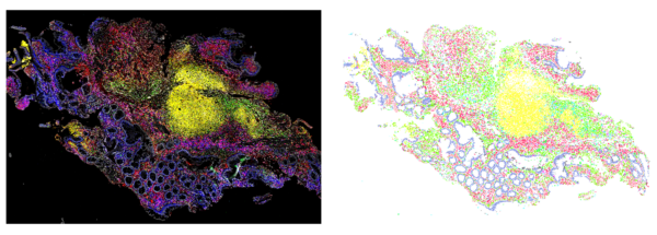
Computer vision is used to find cells in a high-content image of an immune response in the colon (left). In the right, each dot is a cell found by the computer, with different colors encoding different immune cell and colon cell types.
Once we have this detailed map of where all of the different tissue cells and immune cells are, we can look at differences between these maps in patients who did and did not respond to therapy. In lupus nephritis, we found that a high density of B cells (one specific type of immune cell) was associated with kidney survival – meaning those patients likely responded to therapy. Also, small groups of a specific subset of T cells (a different type of immune cell) meant that a patient’s disease would continue to progress, even when treated with the standard of care.
Studying spatial immunity – or the spatial distribution of immune cells – is only possible with the advent of new computer vision methods, or clever applications of existing ones. AI has not just revolutionized this work, but built the foundations for it. As we create better models for mapping immune cells and their spatial relationships, we’ll continue to learn more about what happens when our immune system malfunctions, and hopefully better prepare therapies for when it does.
This work was supported by the Eric and Wendy Schmidt AI in Science Postdoctoral Fellowship, a program supported by Schmidt Sciences.
Mar 07, 2024
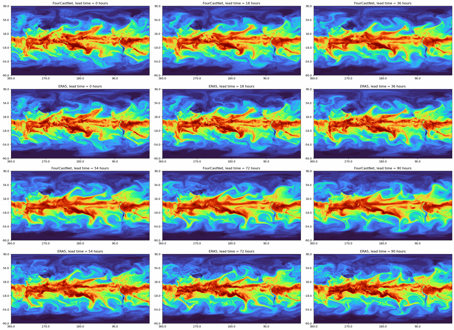
Modeling Chaos using Machine Learning Emulators
Peter Lu, Eric and Wendy Schmidt AI in Science Postdoctoral Fellow
Chaos is everywhere, from natural processes—such as fluid flow, weather and climate, and biology—to man-made systems—such as the economy, road traffic, and manufacturing. Understanding and accurately modeling chaotic dynamics is critical for addressing many problems in science and engineering. Machine learning models trained to emulate dynamical systems offer a promising new data-driven approach for developing fast and accurate models of chaotic dynamics. However, these trained models, often called emulators or surrogate models, sometimes struggle to properly capture chaos leading to unrealistic predictions. In our recent work published at NeurIPS 2023, we propose two new methods for training emulators to accurately model chaotic systems, including an approach inspired by methods in computer vision used for image recognition and generative AI.
Machine learning approaches that use observational or experimental data to emulate dynamical systems have become increasingly popular over the past few years. These emulators aim to capture the dynamics of complex, high-dimensional systems like weather and climate. In principle, emulators will allow us to perform fast and accurate simulations for forecasting, uncertainty quantification, and parameter estimation. However, training emulators to model chaotic systems has proved to be tricky, especially in noisy settings.

An emulator for weather forecasting (top) trained on global weather data (bottom). Source: https://github.com/NVlabs/FourCastNet
One key feature of chaotic dynamics is their high sensitivity to initial conditions which is often referred to colloquially as “the butterfly effect”: small changes to an initial state—like a butterfly flapping its wings—can cause large changes in future states—like the location of a tornado. This means that even a tiny amount of noise in the data makes long-term forecasting impossible and precise short-term predictions very difficult. Accurate forecasts of chaotic systems, like the weather, are fundamentally limited by the properties of the chaos. If this is the case, should we simply give up on making long-term predictions?
The answer is both yes and no. Yes, even with machine learning, we will never be able to predict whether it will rain in Chicago more than a few weeks ahead of time (Sorry to all the couples planning outdoor summer weddings!). No, we should not give up completely because, while exact forecasts are impossible, we can still make useful statistical predictions about the future, such as the increasing frequency of hurricanes due to climate change. In fact, these statistical properties—collectively known as the chaotic attractor—are precisely what scientists focus on when developing models for chaotic systems.
Demonstrating the butterfly effect: Two trajectories from the Lorenz-63 system (a standard simple example of chaos) with slightly different initial conditions that quickly diverge (left) but are statistically similar because they both lie on the same chaotic attractor as seen in the 3D scatter plot (right).
An emulator trained on the Lorenz-63 system with good short-term predictions (1-Step) but poor long-term behavior (Autonomous).
We address this problem by developing new training methods that encourage the emulator to match long-term statistical properties of the chaotic dynamics—which, again, we refer to as the chaotic attractor. We propose two approaches for achieving this:
- Physics-informed Optimal Transport: Choose a set of relevant summary statistics based on expert knowledge: for example, a climate scientist might pick the global mean temperature or the frequency of hurricanes. Then, during training, use an optimal transport metric—a way of quantifying discrepancies between distributions—to match the distribution of the summary statistics produced by the emulator to the distribution seen in the data.
- Unsupervised Contrastive Learning: Automatically choose relevant statistics that characterize the chaotic attractor by using contrastive learning, a machine learning approach initially developed for learning useful image representations for image recognition tasks and generative AI. Then, during training, match the learned relevant statistics of the emulator to the statistics of the data.
The distinction between the two methods lies primarily in how we choose the relevant statistics: either we pick (1) based on expert scientific knowledge or (2) automatically using machine learning. In both cases, we train emulators to generate predictions that match the long-term statistics of the data rather than just short-term forecasts. This results in much more robust emulators that, even when trained on noisy data, produce predictions with the same statistical properties as the real underlying chaotic dynamics.
The best we can hope for when modeling chaos is either short-term forecasts or long-term statistical predictions, and emulators trained using the newly proposed methods give us the best of both worlds. Emulators are already being used in a wide range of applications such as weather prediction, climate modeling, fluid dynamics, and biophysics. Our approach and other promising recent developments in emulator design and training are bringing us closer to the goal of having fast, accurate, and perhaps even interpretable data-driven models for complex dynamical systems, which will help us answer many basic scientific questions as well as solve challenging engineering problems.
Paper citation:
Jiang, R., Lu, P. Y., Orlova, E., & Willett, R. (2023). Training neural operators to preserve invariant measures of chaotic attractors. Advances in Neural Information Processing Systems, 36.
This work was supported by the Eric and Wendy Schmidt AI in Science Postdoctoral Fellowship, a program supported by Schmidt Sciences.
Feb 29, 2024

The AI-Powered Pathway to Advanced Catalyst Development
Rui Ding, Eric and Wendy Schmidt AI in Science Postdoctoral Fellow
In the quest for sustainable energy, the materials that drive crucial reactions in fuel cells and other green technologies are pivotal. At the University of Chicago and Argonne National Lab, a novel approach is being pioneered to discover these materials not through traditional experimentation but by mining the rich data from scientific literature using artificial intelligence (AI) and machine learning (ML). This method is not merely about digesting existing knowledge—it’s about predicting the future of green hydrogen energy production by identifying the most promising catalyst materials for boosting the processes.
This innovative work represents a notable shift in the approach to scientific discovery. By leveraging AI and the extensive information in scientific publications, the research team is accelerating the development of new materials, contributing to the advancement of clean energy technologies.
The Details:
The process starts with an advanced web crawler, which could automatically browse through internet academic databases. It navigates through scientific abstracts, extracting chemical data with precision. This crawler uses Python and specialized packages to translate scientific findings into a digital format that AI can analyze. It’s akin to training a robot to become an expert in scientific literature, resulting in a vast, rich database created efficiently.
Once the crawler has extracted this useful information, the next step uses ML, where algorithms are trained on this data to predict the performance of various materials in electrocatalytic processes. The researchers employ a method known as transfer learning, traditionally used in fields like natural language processing, to apply insights from one chemical domain to another. For example, it is like adopting a skill set from one discipline to excel in another, enhancing the AI’s predictive capabilities.
For the above mentioned whole ML-guided automated workflow, the researchers coined the acronym “InCrEDible-MaT-GO” for the proposed workflow to promote and remember the workflow techniques. Similar to the famous machine intelligence “AlphaGO,” it is expected to contribute to human society in the future by assisting discovery and obtaining new knowledge on “incredible materials” for researchers in various systems and tasks.
The Impact:
This strategy goes beyond expediting the discovery process; it’s about enhancing the precision of scientific prediction. By integrating the web crawler’s data with the predictive prowess of AI, the team can conceptualize new materials that are theoretically optimal, even before they are even physically produced in the lab.
This work has already made notable breakthroughs. For example, the theoretical prediction of an Ir–Cr–O system for oxygen evolution reactions, a vital component of water-splitting technologies. This material was not previously known but was later validated through experimental work, showcasing the predictive model’s potential.
The Excitement:
This research represents a significant stride in material science. AI’s role in interpreting scientific literature and predicting experimental outcomes is a sophisticated addition to the researcher’s toolkit. The “InCrEDible-MaT-GO” workflow exemplifies integrating data science, chemistry, and computer science, addressing some of the most challenging questions in energy research.
As new materials emerge in the energy sector, it’s essential to recognize the role of AI and digital data mining in these advancements. The future of material discovery is evolving, with AI playing a central role in bridging the gap between theoretical prediction and experimental validation.
Additional Resources:
This work was supported by the Eric and Wendy Schmidt AI in Science Postdoctoral Fellowship, a program supported by Schmidt Sciences.
Feb 22, 2024
Automated Material Discovery for More Sustainable Plastics: Describing Polymer Chemistry for Human and Machine
Ludwig Schneider, Eric and Wendy Schmidt AI in Science Postdoctoral Fellow
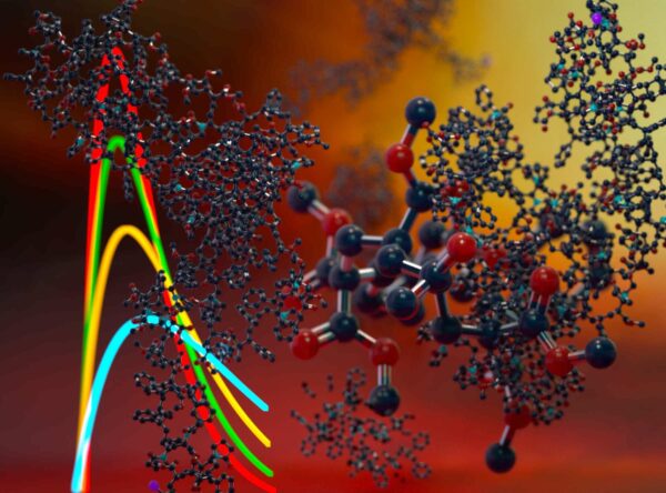
Plastics are a double-edged sword for our environment. Every year, about 500 million tons of plastic are produced, most of which originate from petrochemical sources and end up as waste. Not only does this immense volume of plastic not decompose for centuries, but it also frequently escapes proper disposal, leading to environmental pollution. A stark example is the Great Pacific Garbage Patch, a massive accumulation of plastic in the Pacific Ocean. To put this pollution in perspective, if this patch were made entirely of typical 10-gram shopping bags, it would amount to approximately 10 billion bags, exceeding the human population on Earth.
However, it’s crucial to recognize that not all plastics are inherently harmful. They are incredibly versatile and economical, finding use in everything from everyday clothing and packaging to essential roles in micro-electronics, medical devices, and even battery electrolytes. Our goal, therefore, isn’t to eliminate plastics altogether but to explore sustainable alternatives and rethink our reliance on single-use items.
Sustainable Solutions
The path forward involves making plastics more sustainable. This could be achieved by using plant-based materials, ensuring compostability, or improving recyclability. Significant scientific progress has been made in developing such materials. However, the challenge doesn’t end with sustainability; these new materials must also functionally outperform their predecessors. A notable example is the case of Sunchips’ compostable bags, which, despite being environmentally friendly, were rejected by consumers due to their loud crinkling sound. This illustrates the need for sustainable plastics to meet both environmental and functional standards.
To address this challenge, science is rapidly advancing in the exploration of new materials through automated experimentation, computer simulations, and machine learning. However, these methods require a universal language to describe polymeric materials understandable to both computers and human scientists.
This brings us to the core of what makes plastics unique: polymers. Derived from the Greek words ‘πολύς’ (many) and ‘μέρος’ (parts), polymers are long molecules composed of repeating units called monomers. For instance, simplified polyethylene, the material of common shopping bags, is essentially a long chain of carbon atoms.
Visualizing the structure of a polymer like polyethylene can be straightforward for someone with a chemistry background. A basic representation using text characters, with dashes indicating covalent bonds between carbon (C) and hydrogen (H) atoms, looks like this:
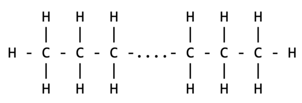
This representation, while instructive for humans, poses a challenge for computers, especially due to its two-dimensional nature. By simplifying the notation and assuming implicit hydrogen bonds, we can transform it into a one-dimensional string more comprehensible to computers:
CCC….CCC
From SMILES Notation to BigSMILES
Expanding this concept leads us to SMILES (Simplified Molecular Input Line Entry System), a widely-used notation for small molecules. However, traditional SMILES doesn’t address the varying lengths of polymers, as a real polymer chain consists of thousands of carbon atoms. Writing them all out would be impractical and overwhelming.
This challenge is elegantly solved by a notation specifically designed for polymers, known as BigSMILES. It represents the repeating nature of monomers in a compact and understandable form. For instance, a simplified version of polyethylene can be represented as:
{[] [$]CC[$] []}
This format not only makes it easier for humans and machines to interpret but also allows for more detailed specification of connections and types of monomers, reflecting a wide range of realistic polymeric materials.
Representing Molecular Weight Distribution
One crucial aspect not yet addressed is the variation in the length of polymer chains in a material, known as the molecular weight distribution. This is where the generative version of BigSMILES, G-BigSMILES, comes into play. It allows the specification of molecular weight distributions, as demonstrated in the following example:
{[] [$]CC[$] []}|schulz_zimm(5000, 4500)|
Here, the Schulz-Zimm distribution is used to describe the average chain lengths in terms of molar masses (M_w and M_n). Here the molar mass is a description of how long the polymer chains are i.e. how many monomers are repeated to compose the chain molecule.
Closing the Loop: From Notation to Material Exploration
With G-BigSMILES, we can now comprehensively describe polymeric materials in a way that’s both human-readable and machine-processable. Our Python implementation allows for the generation of molecular models based on these descriptions, facilitating the exploration of material properties through computer simulations.
Real-world polymeric materials are often more complex, involving branched chains or multiple monomer types. For more in-depth examples, readers are encouraged to consult our publication and GitHub repository.
Looking Ahead: AI-Driven Material Discovery
The next step in our project involves enhancing the interpretability of G-BigSMILES for machines. By translating these notations into graph structures, we aim to enable AI algorithms to suggest new material compositions. The goal is to ensure that these suggestions are not only chemically valid but also optimized for performance, paving the way for more efficient and sustainable material discovery.
This work was supported by the Eric and Wendy Schmidt AI in Science Postdoctoral Fellowship, a program supported by Schmidt Sciences.
Feb 15, 2024

Unlocking the Potential of Lithium Batteries with New Electrolyte Solutions
Ritesh Kumar, Eric and Wendy Schmidt AI in Science Postdoctoral Fellow
Imagine a world where your smartphone battery lasts for days, electric cars charge faster and drive longer, and renewable energy storage is more efficient. This isn’t a distant dream but a possibility being unlocked by groundbreaking research in lithium metal batteries. The key? A novel electrolyte solution that promises to revolutionize how these batteries operate.
Rechargeable lithium batteries are a cornerstone of modern portable electronics, offering a reliable power source for a wide range of devices. At their core, these batteries consist of three key components: an anode, a cathode, and an electrolyte that enables the flow of lithium ions between the anode and cathode during charging (that converts chemical energy into the desirable electrical energy) and discharging (electrical to chemical energy) cycles. The unique chemistry of these batteries allows them to be recharged repeatedly, making them both efficient and environmentally friendly compared to single-use alternatives. This ability to efficiently store and release electrical energy is what has propelled lithium batteries to the forefront of energy storage technology. The specific variant of lithium batteries that ubiquitously powers all electronic gadgets and electric vehicles (EVs) is called a lithium-ion battery. A lithium-ion battery consists of graphite (a form of carbon, the other popular form of carbon you may know as diamond!) as anode and a ceramic solid (mostly contains metal, lithium, and oxygen) and the electrolyte consists of salts (not the one you use in your soup!) dissolved in organic liquids. Their widespread adoption is due to their high energy density (energy stored in a battery per weight) and long life. However, as we push the boundaries of technology and seek more sustainable and efficient energy solutions, the limitations of lithium-ion batteries become apparent. For example, the driving range of EVs is currently limited by the amount of lithium that can be stored in graphite anode in the lithium-ion batteries. This is where the next generation of batteries, such as lithium metal batteries (LMBs), comes into the picture. LMBs promise even higher energy densities, potentially doubling that of standard lithium-ion batteries as they use lithium metal instead of graphite as the anode, and offer faster charging times. This makes them particularly attractive for applications requiring more intensive energy storage, like long-range EVs and more efficient integration with renewable energy sources.
However, their widespread use of LMBs is hampered by two major challenges. The first major challenge lies in the selection of electrolyte, which is crucial for enabling the flow of lithium ions and hence in the generation of electrical energy. The traditional electrolytes used in lithium ion batteries show increased reactivity towards lithium metal anode. They often fail to support the efficient movement of lithium ions and contribute to the rapid degradation of the lithium electrode. This incompatibility significantly hinders the battery’s performance and lifespan.
The second challenge is the uneven deposition of lithium during the charging process (when lithium ions get transported to the anode they get deposited as lithium metal). This unevenness often results in the formation of lithium ‘dendrites,’ needle-like structures that can grow through the electrolyte layer. These dendrites not only reduce the efficiency and lifespan of the battery but also pose significant safety risks. They can create short circuits within the battery, leading to potential failures or, in extreme cases, safety hazards.
The exciting news? We have developed a new type of electrolyte solvent, the fluorinated borate esters, which dramatically enhances the performance and safety of lithium metal batteries, in a recent work published in the Journal of Materials Chemistry A.
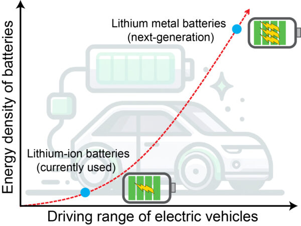
Figure: Development of next-generation batteries such as lithium metal batteries can significantly increase the driving range of current electric vehicles by manyfold. The main bottleneck to the realization of such next-generation batteries is the lack of suitable electrolytes.
Our research team (Amanchukwu Lab) experimentally synthesized a novel electrolyte called tris(2-fluoroethyl) borate (TFEB), a fluorinated borate ester, and investigated for compatibility with LMBs through a series of experimental battery cycling tests. While our cycling tests validated the promising nature of the new electrolytes for LMBs, supporting our initial hypothesis, it presented a challenge: we could not explain our experimental results in terms of molecular behavior and interactions. Understanding these molecular details is not straightforward, as it involves comprehensively analyzing how the electrolyte’s molecules interact at the atomic level. This molecular insight is crucial because it allows us to predict and design the behavior of similar high-performance electrolytes in future experiments. In essence, gaining a clear molecular-level understanding is key to systematically developing electrolytes that can enhance the performance and safety of LMBs. To overcome this challenge, we turned towards cutting-edge computational methods, including quantum chemistry-based density functional theory (DFT) and ab-initio molecular dynamics (AIMD) simulations. These tools allowed us to delve deep into the molecular interactions within the battery, providing insights into the ion solvation (i.e., how lithium ions bond to different molecular components in electrolytes that ultimately decide their properties) environment and the solubility of lithium salts (this is crucial since electrolytes do not work unless salts dissolve in the organic liquids) in fluorinated borate esters.
The implications of this research are far-reaching. With improved solubility and stability offered by TFEB, LMBs can operate more efficiently and safely, paving the way for their use in a variety of applications, from consumer electronics to electric vehicles. Additionally, this study opens the door for future research where artificial intelligence (AI) and machine learning (ML) can play a pivotal role. The computational methods we used in our current work, while effective in predicting the properties of materials, face a significant limitation: they are computationally intensive. This makes them less feasible for exploring the vast chemical space of potential electrolyte candidates, which is astonishingly large, estimated to be in the order of 10ˆ60 possibilities! Here’s where AI algorithms can make a substantial impact. These advanced technologies have the potential to revolutionize how we approach the discovery of new electrolyte solvents. AI and ML are not just faster; they are capable of analyzing complex patterns and data relationships that are beyond human computational ability. This means they can predict, simulate, and optimize the properties of new electrolyte materials much more quickly and accurately than traditional methods. By leveraging AI, we can dramatically speed up the discovery process, potentially leading to breakthroughs in the development of more efficient and sustainable energy storage solutions. Our team is excited to be at the forefront of this innovation. We are actively exploring the use of AI and ML algorithms to tackle this grand challenge.
In summary, this research is not just about improving batteries; it’s about taking a significant step towards a more sustainable and technologically advanced future. With these advancements, the dream of long-lasting, safe, and efficient batteries is closer than ever.
This work was supported by the Eric and Wendy Schmidt AI in Science Postdoctoral Fellowship, a program supported by Schmidt Sciences.
